Time series forecasting involves analyzing data points collected or recorded at time-ordered intervals to predict future values. This technique is widely used in business for financial planning, inventory management, demand forecasting, and capacity planning.
Understanding the components of time series and applying appropriate forecasting models with accuracy assessments are fundamental to deriving reliable predictions.
Time Series Components
Time series analysis relies on separating data into meaningful components. The points below highlight trend, seasonality, cyclical behavior, and noise to enhance pattern recognition and forecasting.
1. Trend: Represents the long-term movement or direction in the data, either increasing or decreasing, reflecting structural changes or growth.
2. Seasonality: Refers to regular, repeating patterns at fixed intervals, such as daily, weekly, monthly, or yearly variations. For example, retail sales often peak during holiday seasons.
3. Cyclical Patterns: Longer-term fluctuations not as regular as seasonality, often tied to economic cycles lasting several years.
4. Noise: Irregular or random variations that cannot be explained by the other components.
Breaking data into these components helps isolate patterns and improves forecast precision.
Forecasting Methods
Accurate forecasting requires choosing the right method for the data at hand. The key techniques below illustrate how smoothing, trend capture, and seasonal adjustments improve predictive performance.
1. Moving Averages: Smooth out short-term fluctuations by averaging data points over a defined period. Simple and easy but less responsive to recent changes.
2. Exponential Smoothing: Assigns exponentially decreasing weights to older observations, capturing trends more effectively than moving averages.
3. Variants like Holt’s Linear and Holt-Winters methods incorporate trends and seasonality, respectively, for more accurate forecasting of complex series.
These techniques are widely used due to their balance of simplicity and effectiveness.
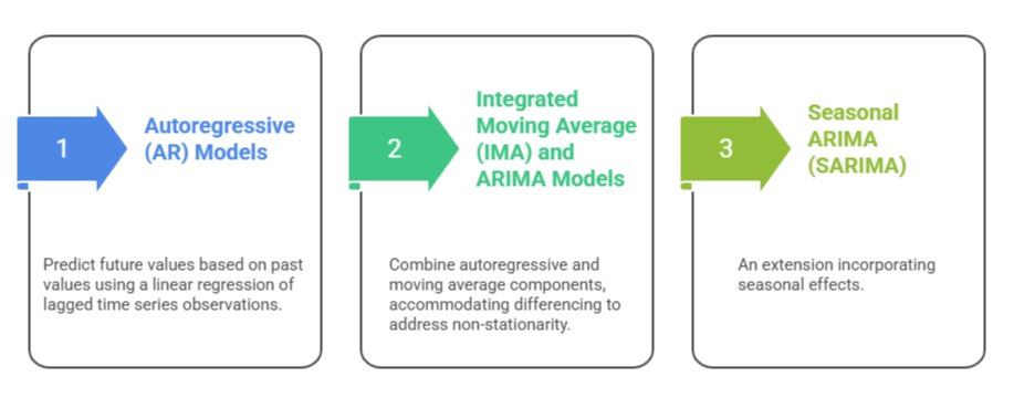
Autoregressive Models and Advanced Time Series Techniques
To model complex time series effectively, analysts use a range of techniques from AR to SARIMA and BSTS. The points below summarize methods that enhance flexibility and forecasting precision.
 Advanced models like Bayesian Structural Time Series (BSTS) and Tbats account for multiple seasonalities and complex patterns.
These advanced models offer higher flexibility and accuracy, especially for intricate data behaviors.
Forecast Accuracy Assessment and Model Comparison
Forecast accuracy assessment helps identify the best models for decision-making. The following points describe error metrics, bias evaluation, cross-validation, and model comparison to improve predictive reliability.
Metrics include:
1. Mean Absolute Error (MAE): Average absolute differences between predicted and actual values.
2. Root Mean Squared Error (RMSE): Penalizes larger errors more than MAE.
3. Mean Absolute Percentage Error (MAPE): Expresses errors as percentages, useful for interpretability.
Forecast bias is assessed to detect systematic over- or under-prediction, ensuring model outputs are reliable. Models are compared using accuracy metrics, simplicity (parsimony), and relevance to the business context.
Cross-validation techniques are employed to ensure that models generalize well to unseen data. Overall, evaluating forecast accuracy supports dependable, data-driven recommendations for business strategy.

Class Sessions
Sales Campaign

We have a sales campaign on our promoted courses and products. You can purchase 1 products at a discounted price up to 15% discount.