Variance and Standard Deviation

Knowing the center of your data through the mean or median is a good starting point, but it is only half the picture. Two datasets can have the exact same mean yet look completely different in terms of how their values are spread out.

Consider two classes of students — both with an average score of 70. In Class A, every student scored between 65 and 75. In Class B, scores ranged from 20 to 100. The mean tells you nothing about this difference.

This is where Variance and Standard Deviation come in. These are measures of spread or dispersion, they quantify how far data points are from the mean, giving you a complete and honest picture of your data's behavior.

Why Spread Matters

Understanding spread is just as important as understanding the center. In business, finance, healthcare, and engineering, the variability in data often carries more decision-making weight than the average alone.

1. A company with consistent monthly sales has low variance — predictable and stable.

2. A company with wildly fluctuating monthly sales has high variance — unpredictable and risky.

3. In manufacturing, low variance in product dimensions means quality and precision.

4. In finance, high variance in stock returns signals high risk.

The mean tells you where data is centered. Variance and standard deviation tell you how reliable that center actually is.

Variance — Measuring Average Spread

Variance measures the average squared distance of each data point from the mean. Squaring the differences ensures that negative and positive deviations do not cancel each other out, and it also amplifies larger deviations, giving more weight to values that are further from the mean.

Population Variance Formula:

Sample Variance Formula: ​

The difference between the two is the denominator — population variance divides by N (total population size), while sample variance divides by n-1. The n-1 adjustment, known as Bessel's correction, compensates for the fact that a sample tends to underestimate the true population spread.

Example Calculation:

Given scores: 60, 70, 80, 90, 100 → Mean = 80

The limitation of variance — Because differences are squared, the result is in squared units (e.g., squared dollars, squared points), making it difficult to interpret directly in the context of the original data. This is exactly why standard deviation is used alongside it.

Standard Deviation — Variance in Readable Units

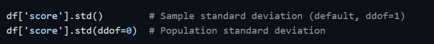
Standard deviation is simply the square root of variance. Taking the square root brings the measure back to the original unit of the data — making it directly interpretable and far more practical for communication and analysis.

Population Standard Deviation:

Sample Standard Deviation:       

Using the same example above:                            

This means that, on average, each student's score deviates from the mean by approximately 15.81 points — a statement that is immediately meaningful and easy to understand.       

Interpreting Standard Deviation

Standard deviation becomes most powerful when used to describe how data is distributed around the mean — particularly in normally distributed data, where the Empirical Rule applies.

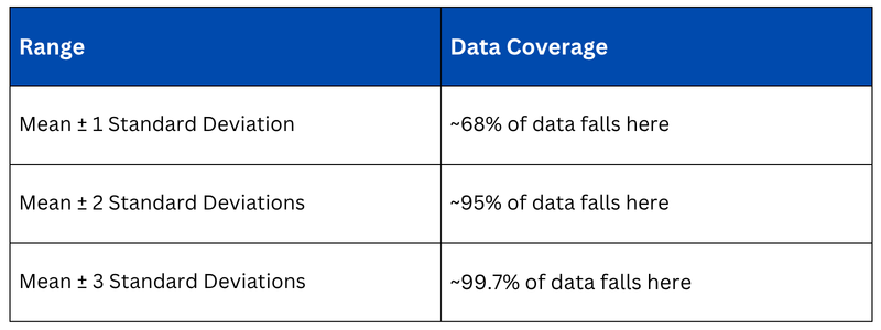
This rule, also known as the 68-95-99.7 Rule, is extremely practical. For example, if the average salary in a company is $60,000 with a standard deviation of $8,000, then approximately 95% of employees earn between $44,000 and $76,000. Any salary beyond $84,000 (3 standard deviations) would be considered statistically unusual — a potential outlier.

Variance vs. Standard Deviation — Key Differences

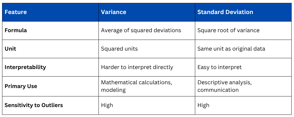Both are sensitive to outliers — a single extreme value increases both measures significantly. This is why always checking for outliers before reporting variance or standard deviation is important.

Computing Variance and Standard Deviation in Python

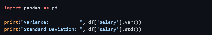
For a full statistical summary that includes standard deviation alongside mean and quartiles:

The .describe() output places the standard deviation (std) directly next to the mean, making it immediately easy to judge whether the mean is a reliable representative of the data or whether high spread makes it less trustworthy.

Visualizing Spread

Numbers alone describe spread, but visuals make it tangible and immediately understandable.

1. A histogram shows the width of the distribution — wider spread means higher standard deviation.

2. A box plot displays the interquartile range and whiskers, directly reflecting data spread.

3. Overlaying a mean line and ±1 std band on a distribution plot gives an instant visual of where most data sits.

import matplotlib.pyplot as plt

mean = df['salary'].mean()

std = df['salary'].std()

plt.hist(df['salary'], bins=30, color='steelblue', edgecolor='black', alpha=0.7)

plt.axvline(mean, color='red', linestyle='--', label=f'Mean: {mean:.0f}')

plt.axvline(mean + std, color='orange', linestyle='--', label=f'+1 STD: {mean+std:.0f}')

plt.axvline(mean - std, color='orange', linestyle='--', label=f'-1 STD: {mean-std:.0f}')

plt.legend()

plt.title('Salary Distribution with Mean and Standard Deviation')

plt.show()