Introduction to Jupyter Notebook Interface

Jupyter Notebook has revolutionized how data analysts and scientists work with code.

Unlike traditional programming environments where you write entire scripts before seeing results, Jupyter allows you to work interactively—writing small pieces of code, running them immediately, and seeing outputs right away.

This interactive approach makes it perfect for data exploration, learning, and presenting findings. 

Understanding the Dashboard

When you first launch Jupyter Notebook, you land on the dashboard—your control center for managing notebooks and files.

Dashboard Layout

The dashboard displays three main tabs at the top:

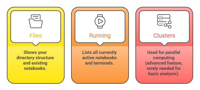
The Files tab is where you'll spend most of your time. It functions like a file explorer, showing folders, notebooks (.ipynb files), and other documents in your current directory.

Key Actions from the Dashboard

You can perform several important tasks directly from this interface:

1. Create new notebooks: Click "New" → "Python 3"

2. Upload files: Use the "Upload" button to add datasets

3. Create folders: Click "New" → "Folder" to organize your work

4. Navigate directories: Click on folder names to browse

5. Rename items: Select the checkbox next to a file and click "Rename"

6. Delete items: Select files and click the trash icon

Think of the dashboard as your project workspace, keep it organized, and your analysis work becomes much smoother.

Anatomy of a Notebook

Once you create or open a notebook, you enter the main working environment. Understanding its components is essential for productive work.

The Notebook Header

At the very top, you'll see:

1. Notebook name: Click "Untitled" to rename your notebook.

2. Last checkpoint: Shows when the notebook was last auto-saved.

3. Kernel indicator: A circle that indicates whether code is running (filled) or idle (empty).

The Menu Bar

The menu bar contains dropdown menus similar to other applications:

The Toolbar

Below the menu bar sits the toolbar with quick-access buttons for common operations:

1. Save icon: Manually save your work (Jupyter also auto-saves periodically)

2. + button: Insert a new cell below the current one

3. Cut, copy, paste icons: Manipulate cells

4. Up/down arrows: Move cells up or down

5. Run button: Execute the current cell

6. Stop button: Interrupt code execution

7. Restart button: Restart the kernel

8. Cell type dropdown: Switch between Code and Markdown

These buttons provide faster access to frequently used functions compared to navigating through menus.

Working with Cells

Cells are the fundamental building blocks of Jupyter notebooks. Every piece of code or text you write lives inside a cell.

Cell Types

Jupyter supports several cell types, but you'll primarily use two:

1. Code Cells (Default)

Code cells contain Python code that gets executed when you run them. After execution, outputs appear directly below the cell, including:

1. Text output from print statements.

2. Data tables from Pandas DataFrames.

3. Visualizations from Matplotlib or Seaborn.

4. Error messages if something goes wrong.

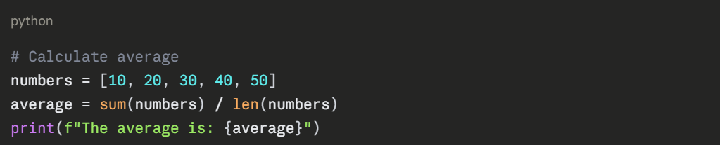
Example of a code cell:

2. Markdown Cells

Markdown cells contain formatted text for documentation, explanations, and notes. They support:

1. Headings using #, ##, ###

2. Bold text with **text**

3. Italic text with *text*

4. Bullet lists using - or *

5. Numbered lists using 1., 2., etc.

6. Links: [text](url)

7. Images: 

Markdown cells help you create narrative around your analysis, making notebooks self-documenting.

Cell Execution

Understanding how to execute cells efficiently is crucial:

1. Run current cell: Press Shift + Enter (moves to next cell)

2. Run and stay: Press Ctrl + Enter (stays in current cell)

3. Run and insert new: Press Alt + Enter (creates new cell below)

4. Run all cells: Menu → Cell → Run All

5. Run cells above: Menu → Cell → Run All Above

6. Run cells below: Menu → Cell → Run All Below

Each code cell has an execution counter displayed as In [n]: where n indicates the order of execution. This helps you track which cells have run and in what sequence.

Cell Modes: Command vs. Edit

Jupyter operates in two distinct modes, and understanding the difference prevents confusion.

Edit Mode (Green border)

Active when you're typing inside a cell. The cell border turns green, indicating you can modify its contents. You enter edit mode by:

1. Clicking inside a cell.

2. Pressing Enter on a selected cell.

In edit mode, keyboard shortcuts don't work—letters you type appear as text or code.

Command Mode (Blue border)

Active when you're selecting or manipulating cells as units. The cell border turns blue. You enter command mode by:

1. Pressing Esc while in edit mode.

2. Clicking outside the cell text area.

In command mode, keyboard shortcuts become powerful tools for navigation and cell manipulation.

Essential Keyboard Shortcuts

Mastering shortcuts dramatically increases your productivity. Here are the most valuable ones:

Command Mode Shortcuts (Blue border - press Esc first)

Edit Mode Shortcuts (Green border - inside a cell)

Universal Shortcuts (Work in both modes)

To view the complete shortcut list, press H in command mode or go to Help → Keyboard Shortcuts.

The Kernel: Your Python Engine

The kernel is the computational engine that executes your code. Understanding how it works helps you troubleshoot issues.

Kernel States

Idle: Ready to execute code (empty circle icon).

Busy: Currently running code (filled circle icon).

Dead: Kernel has crashed or been terminated.

Common Kernel Operations

Interrupt the Kernel

If code runs longer than expected or enters an infinite loop, click the stop button or use Kernel → Interrupt. This stops execution without losing your variables.

Restart the Kernel

Use Kernel → Restart to clear all variables and start fresh. This is helpful when:

1. Variables are in an unexpected state.

2. You want to test if code runs from scratch.

3. Memory usage becomes too high.

Restart and Run All

Kernel → Restart & Run All restarts the kernel and executes all cells from top to bottom. This ensures your analysis runs reproducibly from a clean state.

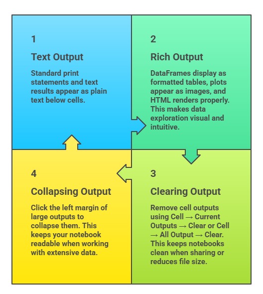
Working with Output

Jupyter handles various output types intelligently, displaying them appropriately.

Saving and Exporting Work

Jupyter provides flexible options for saving and sharing your analysis.

1. Auto-save: Notebooks auto-save periodically (default every 120 seconds). You'll see "Last Checkpoint" timestamp in the header.

2. Manual Save: Click the save icon or press Ctrl + S (Cmd + S on Mac) to save immediately.

3. Export Formats

File → Download as offers multiple formats:

Notebook (.ipynb): Native format for sharing with other Jupyter users

Python (.py): Extract code only, removing outputs and markdown

HTML: Creates standalone webpage viewable in any browser

PDF: Professional document format (requires additional setup)

Markdown: Text-based format for documentation

Each format serves different purposes—use HTML for stakeholder presentations, Python for code sharing, and .ipynb for collaborative analysis.

Best Practices for Using Jupyter

Following these guidelines ensures your notebooks remain organized and effective:

Organization

1. Use markdown cells to create section headers and explain your thinking.

2. Group related code into single cells when logical.

3. Keep cells focused on one task each.

Documentation

1. Add comments within code for technical details.

2. Use markdown cells for high-level explanations.

3. Include data sources and assumptions.

Reproducibility

1. Run "Restart & Run All" before sharing to verify everything executes in order.

2. Avoid relying on variables from cells executed out of sequence.

3. Clear outputs before committing notebooks to version control.

Efficiency

1. Learn and use keyboard shortcuts regularly.

2. Close unused notebooks to free memory.

3. Restart the kernel periodically during long sessions.