Machine learning models rely heavily on efficient optimization methods to achieve stable convergence, reduce training time, and enhance predictive performance.
As datasets become larger and architectures grow deeper, classical gradient descent methods often struggle with slow progress, oscillation, and complex loss landscapes.
Advanced optimization techniques overcome these challenges by incorporating adaptive learning schedules, momentum-driven updates, curvature information, and intelligent parameter adjustments.
These methods enable modern ML systems to navigate irregular error surfaces, escape shallow minima, and maintain stability even in high-dimensional spaces.
Gradient Descent with Momentum
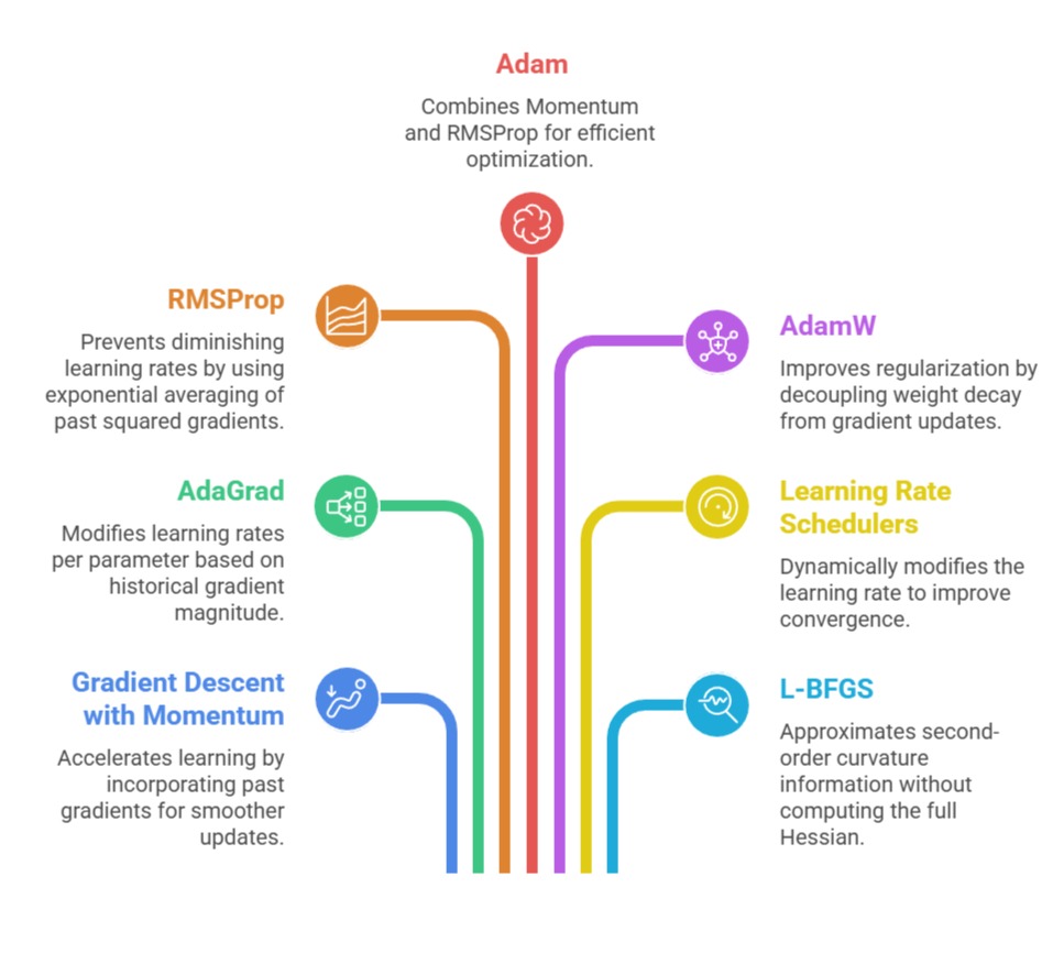
Momentum-augmented gradient descent accelerates learning by incorporating a moving average of past gradients, enabling smoother and more directed parameter updates.
Key Points
1. Momentum builds velocity in the direction of consistent gradients, reducing oscillations in steep or curved regions of the loss surface.
2. It helps models pass through narrow valleys more efficiently, especially in networks with deep hierarchies.
3. The technique suppresses noise from mini-batch updates by blending historical and current gradient information.
4. It stabilizes training when facing jagged or uneven terrains, particularly in vision-based deep learning tasks.
5. Momentum acts like physical inertia, allowing the optimizer to traverse slow directions faster than standard GD.
6. It prevents the learning process from becoming stuck in small bumps or flat plateaus.
7. Common extensions like Nesterov Momentum provide additional foresight by anticipating future positions.
Example: In training convolutional neural networks for image classification, momentum significantly speeds up convergence by smoothing updates across high-curvature regions, improving accuracy and reducing training epochs.
Adaptive Gradient Algorithm (AdaGrad)
AdaGrad modifies learning rates per parameter based on historical gradient magnitude, enabling automatic scaling of updates.
Key Points
1. Parameters that frequently receive large gradients get smaller updates, while rarely updated parameters receive larger steps.
2. This is especially beneficial in highly sparse feature spaces such as natural language or recommender systems.
3. The method helps models focus on underrepresented features that traditional optimizers may overlook.
4. AdaGrad accelerates initial learning by allowing rapidly changing parameters to stabilize early.
5. One limitation is its continuously shrinking learning rate, which can eventually halt training.
6. It remains a useful tool when feature imbalance is prominent and gradient frequencies vary widely.
7. Works well for optimizing classifiers using bag-of-words or TF-IDF embeddings.
Example: AdaGrad was used effectively in early NLP models to train word embeddings from corpora where many tokens appear infrequently.
RMSProp (Root Mean Square Propagation)
RMSProp improves on AdaGrad by preventing diminishing learning rates through exponential averaging of past squared gradients.
Key Points
1. RMSProp dynamically adjusts learning rates without allowing them to approach zero prematurely.
2. It focuses on the most recent gradient patterns rather than accumulating all past information.
3. This makes it well-suited for sequential data and time-dependent signals.
4. The algorithm stabilizes updates for parameters influenced by fluctuating or chaotic gradients.
5. It handles non-stationary scenarios where patterns shift over time, such as reinforcement learning tasks.
6. RMSProp often converges faster than AdaGrad in deep networks with complex architectures.
7. Its adaptive behavior ensures balanced progress even in noisy or drifting environments.
Example: RMSProp is widely used in training recurrent neural networks for speech recognition and temporal sequence modeling.
Adam (Adaptive Moment Estimation)
Adam combines the benefits of Momentum and RMSProp by using both first-order momentum (mean of gradients) and second-order momentum (variance of gradients).
Key Points
1. Adam automatically tailors learning rates for each parameter, improving stability across large-scale models.
2. It compensates for noisy gradients, irregular surfaces, and large parameter counts.
3. Bias-correction techniques ensure consistency during the early training phase when estimates are unstable.
4. Adam requires minimal tuning and works reliably across diverse architectures and tasks.
5. It excels in deep learning applications where gradients differ widely across layers.
6. The optimizer handles sparse gradients efficiently, making it strong for NLP and attention-based models.
7. Its versatility has made Adam a default choice in many neural network frameworks.
Example: Transformers like BERT and GPT models use Adam or AdamW to manage millions of parameters during training.
AdamW (Adam with Weight Decay)
AdamW decouples weight decay from gradient updates, improving regularization in modern neural networks.
Key Points
1. Traditional Adam penalizes both weights and gradients, causing suboptimal regularization.
2. AdamW applies weight decay as a separate additive term, preventing parameter drift.
3. This results in more consistent generalization compared to basic Adam.
4. AdamW helps prevent overfitting in large architectures with heavy parameterization.
5. It enhances model robustness when training deep networks prone to parameter explosion.
6. Often paired with learning-rate warmup schedules in large-scale training environments.
7. AdamW leads to sharper convergence and improved test performance.
Example: AdamW is the optimizer of choice in most state-of-the-art vision transformers (ViT) and large-scale NLP systems.
Learning Rate Schedulers
Schedulers dynamically modify the learning rate during training to improve convergence quality.
Key Points
1. Fixed learning rates often lead to inconsistent or unstable convergence patterns.
2. Schedulers reduce rates gradually, allowing training to start aggressively and end precisely.
3. Step decay, cosine decay, and warm restarts create controlled oscillations or steady reductions.
4. They help models escape shallow regions early and fine-tune parameters later.
5. Warmup strategies prevent instability during early updates in deep networks.
6. In large-batch training, schedulers preserve training quality that otherwise deteriorates.
7. They allow long training cycles without suffering from diminishing returns.
Example: Cosine annealing schedules are used in modern vision architectures like ResNet and EfficientNet to achieve smoother convergence.
Second-Order Optimization (L-BFGS)
L-BFGS approximates second-order curvature information without computing the full Hessian matrix.
Key Points
1. It uses previous gradients to estimate how the loss surface bends.
2. Curvature-based updates often lead to more direct paths to minima.
3. L-BFGS is efficient for medium-sized problems with smooth loss functions.
4. It requires fewer iterations than first-order methods but more computation per step.
5. Often used outside deep learning where parameter counts are manageable.
6. Works well in logistic regression, SVM training, and probabilistic models.
7. Provides highly stable convergence on convex or near-convex landscapes.
Example: Optimization of CRFs (Conditional Random Fields) frequently uses L-BFGS due to its precise yet memory-efficient structure.

Class Sessions
Sales Campaign

We have a sales campaign on our promoted courses and products. You can purchase 1 products at a discounted price up to 15% discount.