Regularization plays a decisive role in ensuring that deep neural networks learn patterns that generalize across diverse and unseen data.
As models grow in depth and parameter count, they become increasingly prone to overfitting, memorizing the training data rather than understanding its underlying structure.
Regularization techniques help counteract this by controlling model capacity, introducing constraints, or limiting excessive reliance on certain neurons or weights.
These methods promote smoother optimization paths, stabilize training dynamics, and produce networks that perform robustly outside the training environment.
Among the most widely adopted strategies are dropout, L2 regularization, and early stopping.
Dropout randomly disables activations during training, encouraging the network to develop redundant and independent feature pathways. L2 regularization, often referred to as weight decay, penalizes excessively large weights to maintain balanced and manageable parameter values.
Early stopping halts training based on validation performance, preventing unnecessary updates that could lead to memorization.
Dropout
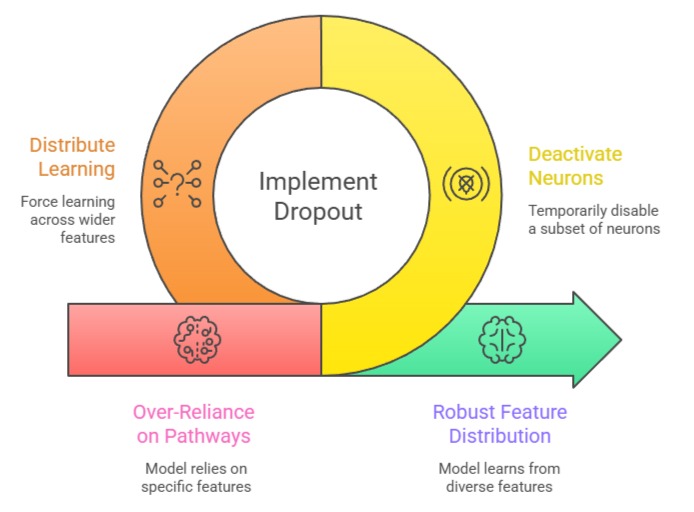
Dropout introduces controlled randomness by temporarily deactivating a subset of neurons during each training iteration.
This prevents the model from relying excessively on specific pathways and forces it to distribute learning across a wider set of features.
Example
1. CNN with dropout 0.5 between dense layers
2. Transformer applying dropout on attention weights
3. LSTM using variational dropout for recurrent units
Advantages
1. Reduces Overfitting by Encouraging Redundant Representations
Dropout compels the network to learn multiple alternative representations of the same concept because neurons cannot depend on their neighbors being active at all times.
This redundancy ensures that even if some features are dropped during training, the model continues producing meaningful outputs.
By distributing importance across many neurons, dropout discourages the formation of brittle feature dependencies that fail under new data.
This creates networks that remain stable across varied inputs and data shifts.
The randomness also acts as a form of ensemble learning, strengthening the diversity of learned representations.
2. Simple Integration With High Effectiveness
Implementing dropout requires only specifying the dropout rate and inserting the layer into the architecture, making it accessible even to beginners.
Despite its simplicity, dropout often leads to noticeable improvements in accuracy without significantly modifying the model design.
Its lightweight nature means it easily complements other regularization methods.
Dropout’s intuitive behavior also facilitates experimentation, allowing practitioners to adjust rates to achieve desired levels of regularization.
Because it operates at the neuron level, it adapts smoothly across feedforward networks, CNNs, and RNNs.
3. Acts as an Implicit Ensemble Technique
Dropout effectively trains multiple “thinned” networks simultaneously by randomly removing neurons in each iteration.
At inference time, the full network acts as an ensemble of these smaller networks, aggregating their predictions.
This ensemble-like effect improves generalization without explicitly training multiple models, saving computational resources.
It increases robustness to noise and unexpected input variations, since the network does not overly rely on specific paths.
By diversifying internal representations, dropout mitigates bias in feature selection and reduces the risk of overfitting to idiosyncrasies in the training set.
4. Adaptable Across Various Architectures
Dropout is not limited to feedforward networks; it can be applied to convolutional layers, recurrent networks, and transformer attention mechanisms.
Variational dropout in RNNs maintains temporal consistency, while dropout on attention layers improves robustness in sequence models.
Its adaptability makes it suitable for a wide range of AI tasks, including NLP, vision, and speech.
This universality allows teams to adopt a single regularization strategy across multiple architectures, simplifying experimentation and improving overall model reliability.
Disadvantages
1. Slower Convergence Due to Noise in Activations
The random removal of neurons introduces noise into the training process, causing each forward pass to behave slightly differently.
This inconsistency forces optimizers to navigate a more irregular loss landscape, often requiring additional epochs to achieve stability.
The variability may also complicate understanding of feature importance, as neuron activations shift from iteration to iteration.
In deeper architectures, this noise can slow down weight updates and prolong the overall training duration.
While beneficial for regularization, the stochastic nature may hinder convergence speed. This trade-off must be accounted for in time-limited or resource-constrained environments.
2. Performance Sensitivity to Dropout Rates
Selecting the wrong dropout rate can harm model performance significantly.
A rate that is too high may erase critical information pathways, preventing the network from forming strong feature detectors.
Conversely, too low a rate may fail to provide sufficient regularization, allowing overfitting to persist.
Tuning dropout values therefore becomes essential, requiring experimentation and validation monitoring.
Different architectures respond uniquely to dropout, making cross-model generalization difficult. These sensitivities make dropout less predictable compared to weight-based methods like L2 regularization.
3. Inconsistent Behavior During Inference if Misconfigured
Dropout layers behave differently during training and inference.
If not properly scaled or handled, activations may not reflect the expected average magnitude, leading to unstable predictions.
Some beginners may forget to switch the network to evaluation mode (model.eval() in PyTorch), causing drastic performance drops during testing.
This discrepancy can introduce subtle bugs and produce misleading validation results. Careful attention is required to maintain consistency between training and inference stages.
4. Not a Substitute for Data Quality or Size
While dropout improves generalization, it cannot compensate for insufficient data, noisy labels, or poor feature representation.
Models trained on limited or biased datasets may still overfit, despite heavy dropout.
Overreliance on dropout may give a false sense of security, leading to neglect of essential practices like data augmentation, proper preprocessing, or acquiring additional training samples.
L2 Regularization (Weight Decay)
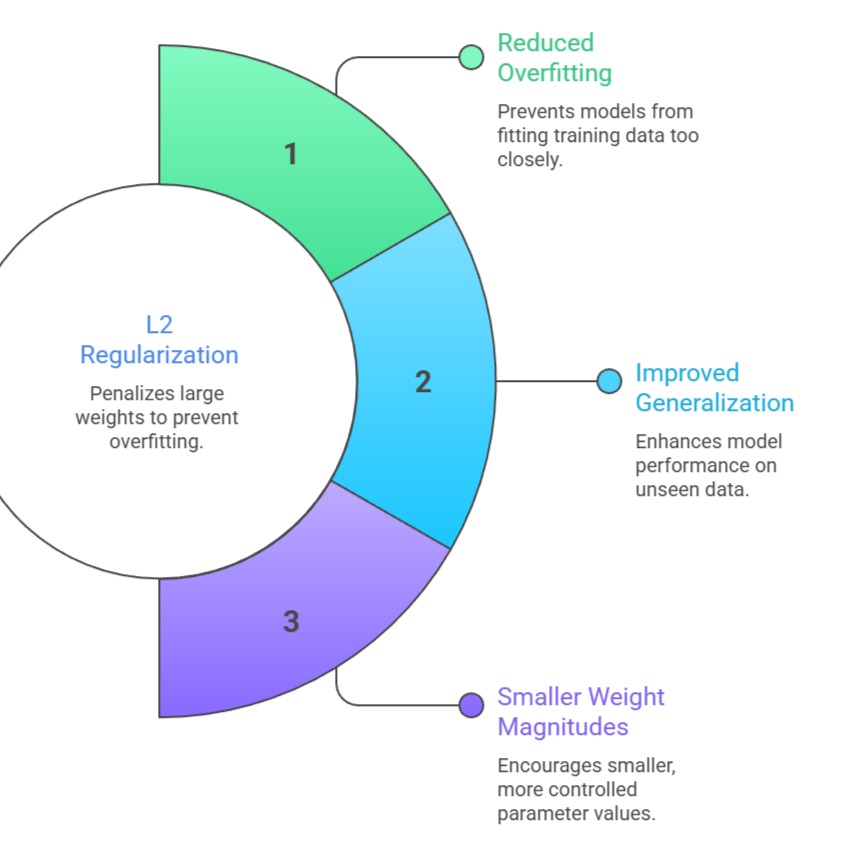
L2 regularization penalizes large weight magnitudes by adding a term proportional to the square of each weight to the loss function.
This encourages the model to maintain smaller, more controlled parameter values.
Example
1. Weight decay 0.0005 in CNN classifiers
2. L2 penalty in logistic regression baseline models
3. AdamW using decoupled weight decay for transformers
Advantages
1. Promotes Smooth and Well-Behaved Weight Distributions
L2 regularization discourages excessive weight growth, which often leads to unstable training dynamics and overfitting.
By nudging weights toward smaller values, it ensures that the model develops smoother decision boundaries that generalize more effectively.
This stabilizing effect allows networks to learn more gradual feature transitions, avoiding abrupt or overly complex patterns that fail on unseen data.
Smaller weights also contribute to improved numerical stability, reducing gradient spikes or oscillations during optimization.
The resulting models typically achieve better calibration and maintain predictable behavior during inference. This creates a more reliable foundation for production-ready systems.
2. Efficient and Computationally Inexpensive
Because L2 regularization simply modifies the loss function with a penalty term, it requires minimal computational overhead.
The implementation is straightforward, highly scalable, and integrates seamlessly with modern optimizers like AdamW. Its deterministic behavior results in consistent outcomes across training runs.
Additionally, L2 regularization improves training smoothness without introducing randomness or architectural modifications.
This makes it ideal for environments where reproducibility and stability are critical requirements.
Its low-cost nature enables application to large or complex models without significantly increasing runtime.
3. Reduces Model Sensitivity to Outliers
By constraining weight magnitudes, L2 regularization prevents any single feature from dominating the model’s predictions.
This produces smoother decision boundaries that are less sensitive to outliers or anomalous samples.
In datasets with noisy labels or extreme values, L2 helps maintain stable predictions and avoids erratic behavior caused by disproportionately large weights.
The result is a model that generalizes more consistently across both typical and edge-case inputs.
4. Complementary to Other Regularization Techniques
L2 regularization integrates well with dropout, batch normalization, and early stopping.
While dropout promotes distributed feature learning and early stopping prevents excessive training, L2 ensures weight control throughout the network.
Combining these methods often results in synergistic effects, producing models with superior generalization performance.
Its deterministic and low-overhead nature makes it easy to layer with other techniques without adding stochasticity or significant computational cost.
Disadvantages
1. Limited Effectiveness for Highly Complex or Deep Models
L2 regularization may not sufficiently address overfitting when the model is excessively large or when data is limited.
In such cases, even well-controlled weights may fail to prevent memorization of training samples. Deep architectures with millions of parameters may still overfit despite moderate or heavy use of L2 penalties.
This limitation becomes particularly evident when datasets exhibit noise or imbalance.
As a result, L2 often must be paired with additional techniques like dropout or data augmentation. On its own, it may not enforce enough structural diversity to combat complex overfitting patterns.
2. Requires Careful Tuning of the Regularization Coefficient
Choosing an overly strong regularization term may restrict the model’s ability to learn meaningful features, leading to underfitting.
A coefficient that is too small may not provide meaningful control over weight behavior.
Tuning this parameter often requires experimenting with multiple values and monitoring validation metrics closely.
Different optimizers respond differently to L2 penalties, adding another layer of complexity.
3. May Slow Convergence if Too Strong
Excessive L2 penalties can overly constrain weights, limiting the network’s ability to learn complex patterns.
This may cause the optimizer to take smaller steps in weight space, slowing convergence and requiring more training iterations.
In highly nonlinear models or deep architectures, strong weight decay may prevent the network from reaching an effective minimum, resulting in underfitting.
Careful tuning of the regularization coefficient is essential to balance generalization and learning efficiency.
4. Uniform Penalty May Not Suit All Layers Equally
Applying the same L2 coefficient across all layers assumes that each layer requires equal regularization, which may not be optimal.
Early layers may benefit from weaker regularization to capture low-level patterns, while deeper layers may require stronger constraints to prevent overfitting.
Uniform weight decay may therefore reduce flexibility and limit performance unless carefully adjusted layer-wise.
This makes L2 less adaptable in heterogeneous or very deep architectures.
Early Stopping
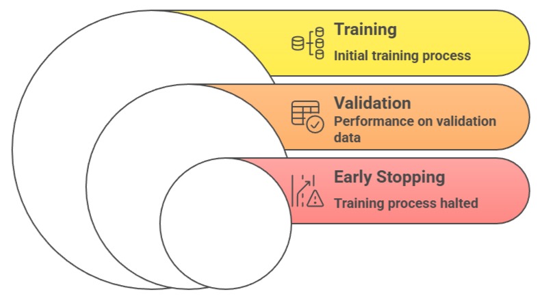
Early stopping halts the training process when validation performance stops improving, preventing the model from overfitting by training beyond the point of optimal generalization.
Examples
1. Stop training when validation loss rises for 5 consecutive epochs
2. Save checkpoints at best validation accuracy
3. Apply early stopping in transformer pretraining to reduce compute
Advantages
1. Prevents Overtraining and Protects Generalization
By monitoring validation loss or accuracy, early stopping identifies when a model begins to memorize training patterns rather than strengthening its generalization capabilities.
This automatic intervention avoids the deterioration of performance caused by unnecessary updates.
Early stopping acts as a safeguard against overly long training sessions that push weights into overfitted regions.
It is particularly useful for models that exhibit rapid early improvements followed by plateaus or fluctuations.
By halting at the right moment, early stopping helps preserve the best-performing version of the model. The result is a network that remains reliable across real-world data.
2. Saves Computational Time and Resources
Early stopping prevents redundant training epochs, reducing GPU usage and overall training time.
This makes it highly valuable in large-scale training environments where full epoch cycles can be expensive.
It also shortens experimentation cycles, enabling faster iteration across architectures or hyperparameter configurations.
This reduced computational demand makes early stopping accessible even for practitioners with limited hardware resources.
It is particularly useful in fast-paced development workflows, where quick validation feedback is beneficial.
3. Reduces Risk of Over-Optimization on Training Data
Early stopping prevents the network from optimizing too aggressively on training data, which can lead to memorization rather than learning useful patterns.
This is particularly important in scenarios with small datasets or highly complex networks, where over-optimization can easily occur.
By stopping training when validation performance plateaus, the model retains its generalization potential without being skewed by training-specific artifacts.
This also provides a safeguard against learning spurious correlations.
4. Works in Tandem With Other Techniques
Early stopping complements other regularization strategies like dropout and L2.
While these methods reduce overfitting by controlling network capacity and weights, early stopping adds a dynamic mechanism to halt training at the ideal point.
This layered approach enhances overall model stability, allowing practitioners to combine static and adaptive regularization for improved performance.
Early stopping is especially useful when computational budgets are limited, as it naturally prevents wasted epochs.
Disadvantages
1. Highly Dependent on Validation Set and Monitoring Strategy
The timing of early stopping relies entirely on validation performance, making it sensitive to noise or fluctuations in validation metrics.
If the validation split is not representative, the model may stop prematurely and fail to reach optimal performance.
Similarly, improper configuration of patience or monitoring frequency may cause early termination or unnecessary continuation.
These sensitivities require careful planning and repeated verification to ensure stability.
Over-reliance on early stopping can mask deeper issues in model capacity or data quality. Poor validation setups can lead to inconsistent results across training runs.
2. Potential Underfitting if Stopped Too Early
If early stopping activates too soon, the model may halt before fully learning essential patterns in the data.
In such cases, the network remains undertrained, producing suboptimal performance on both training and test sets.
This risk increases when validation curves exhibit temporary dips that may not reflect true generalization trends.
As a result, setting patience values and monitoring rules becomes critical.
Practitioners must balance vigilance against premature interruption with the need to avoid prolonged training.
3. Vulnerable to Validation Noise
If the validation set contains noise, fluctuations, or non-representative samples, early stopping may trigger too early or too late.
The model could halt before learning essential patterns or continue training despite clear overfitting.
This dependence on a single validation metric makes early stopping less robust in unstable or small validation splits.
Practitioners often need to use techniques like smoothing or patience intervals to mitigate this issue.
4. Requires Careful Choice of Patience and Frequency
The “patience” parameter (how many epochs to wait before stopping) and the frequency of validation checks are critical.
Too short a patience may halt training prematurely, while too long may reduce the method’s benefits.
Similarly, infrequent validation checks may delay stopping, wasting computation.
Tuning these parameters adds complexity and can affect reproducibility and performance if misconfigured.