Forward propagation, backward propagation, and loss functions together form the learning engine that powers deep neural networks.
Forward propagation is the step where input data is transformed into outputs through multiple layers of weights and activation functions. It represents the model’s attempt to generate meaningful predictions based on its current understanding.
Once the output is produced, a loss function evaluates how far the prediction is from the true target and assigns a numerical value representing the model’s error. This error becomes the foundation for backward propagation.
Backward propagation then uses calculus—specifically, the chain rule—to trace the error backward through the network and compute gradients for each parameter.
These gradients indicate how each weight contributed to the final error, enabling the optimization algorithm to update the model in a direction that reduces future mistakes.
Loss functions, therefore, act as the guiding compass of learning, while the forward and backward passes act as the machinery executing this guidance.
Forward Propagation
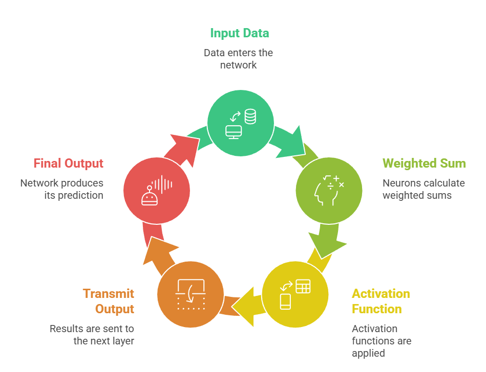 Forward propagation is the stage where data flows from the input layer toward the output layer, undergoing transformations at every step.
Each intermediate layer captures increasingly refined features, allowing the network to make structured predictions based on learned patterns.
Advantages
1. Clear and structured execution flow
The progression of data from input to output follows a fixed and systematic path, making it easy to understand and debug.
Every transformation whether linear or nonlinear is applied sequentially, ensuring the model processes information in a predictable manner.
This structure allows developers to inspect intermediate results, identify where feature extraction may be failing, and refine architectures based on empirical observations.
2. Supports scalable feature learning
As information passes through deeper layers, the network can automatically derive complex patterns without needing handcrafted features.
This scalability enables models to learn low-level and high-level abstractions, supporting sophisticated tasks such as image object detection and language translation.
It removes the dependence on domain-specific manual engineering.
3. Highly optimized for hardware acceleration
Forward propagation operations matrix multiplications, convolutions, and activations are well-suited for parallel execution on GPUs and TPUs.
This synergy between algorithm design and hardware architecture accelerates real-time inference and boosts training speed.
As a result, even very deep models can propagate data efficiently across layers.
Disadvantages
1. Cannot update parameters on its own
Forward propagation only computes outputs; it does not modify weights.
Without backward propagation, the model cannot learn from mistakes, making this step incomplete for training.
This limits its standalone utility to inference scenarios, highlighting the need for gradient-based learning mechanisms.
2. Dependent on weight initialization quality
Poor initialization can cause activations to saturate or explode, which disrupts effective information flow through the network.
If neurons output extreme or stagnant values, later layers receive distorted signals, leading to inaccurate predictions.
This sensitivity means initialization must be carefully chosen to maintain stability.
3. Computational load rises with depth
In very large architectures, executing forward propagation requires extensive memory and processing cycles. Each layer multiplies the cost, making training on CPUs slow and sometimes impractical. This creates a dependency on specialized hardware, impacting accessibility for beginners or small-scale projects.
Example of Forward Propagation
A CNN analyzing an image: pixels → convolution layers → pooling → dense layer → final softmax output.
Backward Propagation
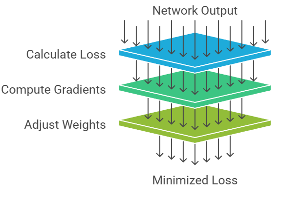
Backward propagation is the process where the network computes gradients of the loss with respect to every parameter.
These gradients determine how much each weight contributed to the error and in which direction it should be adjusted.
Advantages
1. Enables efficient gradient-based learning
Backprop calculates gradients layer-by-layer using shared intermediate results, reducing the computational burden dramatically.
Instead of recomputing derivatives from scratch, it reuses already computed activations, making training deep networks feasible even with millions of parameters.
2. Facilitates continual refinement of the model
Each backward pass updates weights based on the latest loss value, creating a continuous feedback loop between prediction and correction.
Over many iterations, the network gradually shapes its internal representations to match the patterns hidden in the data. This allows deep learning models to improve accuracy steadily.
3. Compatible with diverse architectures and activations
Backprop supports almost every modern architecture—CNNs, RNNs, LSTMs, Transformers—so long as their operations are differentiable.
This flexibility enables innovation in neural network design, allowing researchers to combine unconventional layers while relying on standard gradient flow mechanisms.
Disadvantages
1. Risk of vanishing or exploding gradients
In deep networks, gradients can become extremely small or extremely large as they propagate backward. When gradients vanish, weights barely change, slowing learning to a halt.
When they explode, weights become unstable, causing the model to diverge. Mitigating this requires special activation functions, normalization, or residual connections.
2. High computational and memory demands
Backward propagation requires storing intermediate outputs from the forward pass and calculating derivatives for each layer.
This doubles the computational expense compared to inference and increases memory requirements substantially. Larger models therefore require costly GPU clusters or distributed training systems.
3. Sensitive to hyperparameter choices
Training stability depends heavily on settings such as learning rate, batch size, and gradient clipping thresholds.
Poor choices can lead to oscillating gradients, slow convergence, or complete failure to learn. This sensitivity makes tuning an essential but time-consuming part of model development.
Example of Backpropagation
Updating the weights of a sentiment classifier by computing gradients of the loss w.r.t. embedding vectors and dense layers.
Loss Functions
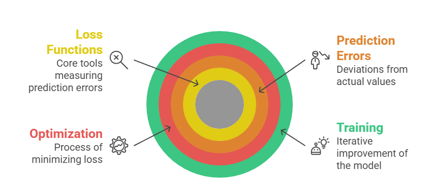
Loss functions are mathematical tools that measure how far the model’s predictions deviate from the actual target values.
They provide the signal that drives optimization during training.
Advantages
1. Establishes a clear learning objective
Loss functions quantify performance in a single value, guiding optimization toward a well-defined goal.
This clarity helps models learn consistently across epochs and ensures that weight updates directly correspond to measurable improvements.
A properly selected loss function makes training stable and targeted.
2. Can be tailored to different problem types
Different tasks require different error metrics—cross-entropy for classification, MSE for regression, triplet loss for embedding learning, etc.
This adaptability allows models to be optimized for the exact behavior expected in real-world scenarios, improving overall task alignment and reliability.
3. Offers meaningful training diagnostics
Monitoring loss values across epochs reveals how well a model is learning.
A steep decline indicates strong early learning, whereas a plateau suggests stagnation.
Sudden spikes can reveal instability or improper hyperparameters. Thus, loss serves as a real-time indicator of training health.
Disadvantages
1. Incorrect choice weakens performance
Choosing an inappropriate loss can misguide the entire learning process.
For example, using MSE for classification produces poor gradient behavior and slows convergence.
Misaligned loss functions also distort gradient direction, preventing the model from learning correct decision boundaries.
2. Vulnerable to extreme outliers
Certain loss functions, such as MSE, heavily penalize large errors.
While sometimes beneficial, this sensitivity can cause instability in datasets with noisy or mislabeled samples.
The model may over-adjust to outliers, harming generalization and producing unreliable predictions.
3. Doesn’t directly represent task metrics
Loss values often do not map directly to real-world accuracy or performance scores.
For instance, lowering cross-entropy does not always guarantee improved precision or recall.
As a result, relying solely on loss may give a misleading impression of true model quality.