Feature Engineering Basics

Feature engineering is one of the most influential stages in the machine learning pipeline, shaping how models interpret and learn from data.

It involves transforming raw information into meaningful representations that expose hidden relationships, patterns, and signals.

Well-designed features can dramatically elevate model performance, reduce training complexity, and address real-world irregularities such as noise, missing values, or inconsistent scales.

In Python, this step often combines domain knowledge, analytical insight, and computational tools—especially those provided by libraries like Pandas, NumPy, and Scikit-learn.

Good feature engineering encompasses several tasks: handling missing values sensibly, encoding categorical variables, creating interaction features, extracting temporal or text-based attributes, scaling numerical fields, and reducing dimensionality when necessary.

Each modification aims to help the model “see” the underlying structure of the dataset more clearly.

Because machine learning algorithms vary in how they interpret data—linear models, tree-based methods, and neural networks rely on different signals—the choice of engineered features must respect the characteristics of both the dataset and the chosen algorithm.

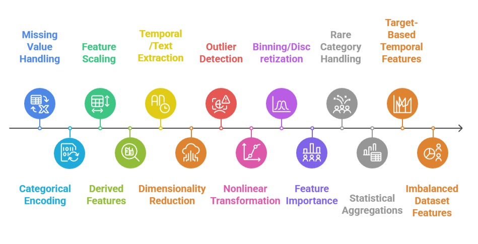
Importance of Feature Engineering

1. Handling and Imputing Missing Values

Missing data can distort model training, weaken relationships, and introduce bias if not treated properly.

Feature engineering begins by identifying the pattern of missingness—whether random or systematic—and applying suitable strategies such as mean/median substitution, regression-based imputation, K-NN filling, or domain-specific rules.

These decisions help maintain data consistency and preserve distribution characteristics.

 For example, in a housing dataset, missing “number of floors” may be imputed with the most common value in the neighborhood.

Proper imputation prevents algorithms from misinterpreting gaps as signals. When paired with flags indicating imputed fields, models can even learn from missingness patterns.

2. Encoding Categorical Variables

Many algorithms require numerical input, making category encoding a critical step.

Techniques like one-hot encoding, label encoding, target encoding, or frequency encoding convert categorical attributes into meaningful numeric forms. The choice depends on cardinality and algorithm type.

 For instance, one-hot encoding works for low-category variables but becomes inefficient for high-cardinality fields, where target encoding may perform better.

Proper encoding ensures that categorical relationships translate accurately into model-interpretable structures, especially for algorithms like logistic regression or SVMs.

3. Feature Scaling and Normalization

Uneven scales can cause distance-based or gradient-based algorithms to misbehave.

Feature scaling techniques—such as standardization, normalization, and min–max scaling—ensure that numerical fields contribute proportionately to the model’s objective function.

 For example, in k-means clustering, unscaled features could cause variables with large ranges (e.g., income) to overshadow smaller ones (e.g., age).

Applying scaling creates uniformity and improves convergence. Tree models may not require scaling, but neural networks and linear models heavily benefit from it.

4. Creating Derived or Interaction Features

New features that combine existing ones often reveal deeper patterns not visible in raw data.

Interaction terms, ratios, polynomial features, and domain-specific transformations can significantly boost performance.

 For example, instead of using “distance” and “time” separately, creating a “speed” variable may directly capture the behavior relevant to the prediction task.

Similarly, polynomial features help linear models approximate nonlinear relationships, expanding their expressive power.

5. Temporal, Text, and Domain-Specific Feature Extraction

Raw timestamps, text fields, or domain-centric attributes usually require transformation to be useful.

Extracting features such as hour of day, sentiment score, keyword presence, or seasonal indicators can drastically improve predictions.

 For instance, in sales forecasting, capturing “day of week,” “holiday flag,” or “promotion period” adds crucial contextual information.

Text data may benefit from token counts, TF-IDF values, embeddings, or n-grams, depending on the model's complexity and the problem’s scope.

6. Dimensionality Reduction and Feature Selection

High-dimensional data may cause overfitting or computational overhead.

Feature selection methods (e.g., mutual information, chi-square tests, L1 regularization) or dimensionality reduction tools (e.g., PCA) streamline the feature space.

 For example, PCA helps when dealing with image or sensor data where variables are correlated.

Reducing dimensionality improves training speed, enhances generalization, and makes models more interpretable—especially in real-time systems.

7. Outlier Detection and Treatment

Outliers can distort statistical relationships and mislead algorithms that rely on distance, error minimization, or gradient calculations.

Feature engineering involves identifying anomalies using methods such as IQR, Z-score thresholds, isolation forests, or visual inspection with boxplots.

Once detected, decisions must be made whether to cap, transform, or remove these outliers depending on the domain.

For example, log-transforming extremely skewed income values reduces their influence while keeping the data intact.

Proper outlier handling ensures models rely on representative patterns rather than extreme aberrations.

8. Feature Transformation for Nonlinear Patterns

Real-world datasets often exhibit nonlinear relationships that linear models cannot naturally capture.

Transformations such as logarithmic, square root, exponential, or Box–Cox scaling reshape data to make relationships more linear or stabilize variance.

For instance, sales volume can be log-transformed to reduce the impact of unusually large orders.

These transformations support more stable model training, reduce skewness, and improve interpretability.

Algorithms like linear regression or SVMs particularly benefit from such engineered feature adjustments.

9. Binning and Discretizing Continuous Variables

Transforming continuous features into bins or categories can simplify relationships or highlight segment-based behavior.

Techniques like equal-width binning, equal-frequency binning, or K-means-based discretization group values into meaningful intervals.

For example, converting age into brackets such as “young adult,” “middle-aged,” or “senior” can reveal patterns invisible in raw numeric form.

Binning reduces noise, helps capture thresholds, and is useful for models requiring interpretable rules such as decision trees or rule-based systems. It also helps mitigate the effect of outliers.

10. Feature Importance Analysis and Iterative Refinement

Feature engineering is iterative, and analyzing feature importance helps refine and enhance the design of features.

Tools like permutation importance, SHAP values, or information gain highlight which attributes are influential.

This enables removal of redundant or weak features while focusing attention on those carrying meaningful predictive power.

For example, if SHAP values show that customer tenure contributes minimally to churn prediction, the feature can be removed or re-engineered into a more informative representation.

This optimization improves performance and reduces model complexity.

11. Encoding Rare Categories and Managing High Cardinality

High-cardinality categorical variables—such as ZIP codes, product IDs, or card types—can create sparse matrices and lead to overfitting.

Specialized encodings like hashing, target encoding, and leave-one-out encoding address this challenge by compressing or approximating category information.

Rare category grouping is another approach, where infrequent categories are merged into an “other” bucket to stabilize learning.

For example, combining seldom-used shipping methods prevents the model from giving undue weight to rare occurrences.

These strategies maintain computational efficiency while preserving predictive strength.

12. Generating Statistical Aggregations

Aggregating numerical fields across categories can reveal structural patterns in the dataset.

Group-by operations calculate features such as mean, median, count, min, max, or variance for each category.

For example, creating a feature representing the average purchase amount per customer segment can uncover behavioral patterns not visible in raw data.

Aggregation is especially powerful in transactional datasets, recommendation systems, and temporal modeling, where grouped behavior signals model-relevant insights.

These features often outperform raw variables due to their inherent smoothing effect.

13. Target-Based Temporal Features

In time-series or sequence-based data, creating lag features, rolling averages, rolling standard deviations, and difference features captures temporal persistence or volatility.

For instance, predicting energy consumption may involve adding a 7-day moving average to represent recent usage trends.

Lag features help models understand seasonal cycles, trends, and dependencies between past and future values.

Temporal features also prevent data leakage when engineered properly with time-aware splits, maintaining the integrity of the modeling pipeline.

14. Feature Construction for Imbalanced Datasets

When working with imbalanced classes, engineered features can help models better separate minority and majority patterns.

Techniques include ratio features, class-prior adjustments, engineered risk scores, and anomaly flags.

For example, in fraud detection, creating a “transaction-to-merchant-frequency” ratio helps highlight unusual user behavior.

These engineered attributes often carry more discriminatory power than raw data, aiding models in handling skewed distributions without relying solely on sampling methods like SMOTE.