Simple AI Project Walkthrough (Prediction Model)

Python fundamentals, data structures, functions, libraries, file handling, and machine learning concepts — comes together in a real AI project. This walkthrough builds a complete, end-to-end Student Pass/Fail Prediction Model from scratch.

Given a student's study hours and attendance percentage, the model will predict whether they will pass or fail. This is a practical supervised classification problem that demonstrates the full AI development pipeline in a clear, beginner-friendly way.

Project Overview

Project Name: Student Pass/Fail Predictor

Problem Type: Binary Classification

Algorithm: Logistic Regression

Features: Study hours, Attendance percentage

Target: Pass (1) or Fail (0)

Libraries: NumPy, Pandas, Matplotlib, Scikit-learn

Step 1 — Import Libraries

Start by importing all the tools needed for the project.

Step 2 — Create the Dataset

In a real project, you would load data from a CSV file. Here, a sample dataset is created directly in code to keep things self-contained and runnable.

python

# Sample student dataset

data = {

    "study_hours":  [1, 2, 2, 3, 4, 4, 5, 5, 6, 6, 7, 7, 8, 8, 9, 9, 10, 1, 3, 6],

    "attendance":   [40, 45, 55, 50, 60, 65, 60, 70, 75, 80, 78, 85, 88, 90, 92, 95, 98, 30, 52, 72],

    "result":       [0, 0, 0, 0, 0, 1, 1, 1, 1, 1, 1, 1, 1, 1, 1, 1, 1, 0, 0, 1]

}

# 0 = Fail, 1 = Pass

df = pd.DataFrame(data)

print(df.head(10))

print("\nResult distribution:")

print(df["result"].value_counts())

Output:

study_hours  attendance  result

0            1          40       0

1            2          45       0

...

Result distribution:

1    13

0     7

Step 3 — Explore the Data

Before building a model, always explore and visualize the data to understand patterns.

python

# Basic statistics

print(df.describe())

# Check for missing values

print("\nMissing values:")

print(df.isnull().sum())

# Visualize — Study Hours vs Attendance coloured by Result

colors = df["result"].map({0: "red", 1: "green"})

plt.figure(figsize=(8, 5))

plt.scatter(df["study_hours"], df["attendance"], c=colors, s=100, edgecolors="black")

plt.xlabel("Study Hours")

plt.ylabel("Attendance (%)")

plt.title("Student Results — Green: Pass | Red: Fail")

plt.grid(True)

plt.show()

The scatter plot immediately reveals the pattern — students with higher study hours and attendance tend to pass. This confirms the features are relevant for prediction.

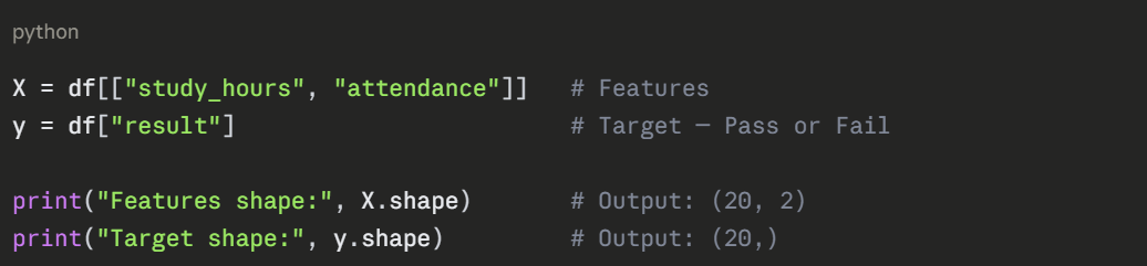
Step 4 — Prepare Features and Target

Separate the input features from the output label.

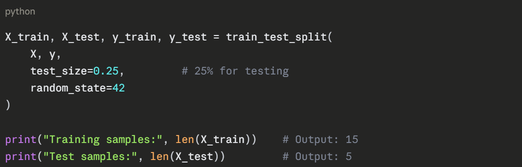
Step 5 — Split into Training and Test Sets

Divide the data so the model trains on one portion and is tested on another it has never seen.

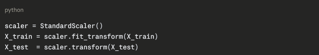
Step 6 — Scale the Features

Standardize the feature values so both study hours and attendance contribute equally to the model.

Step 7 — Train the Model

Create and train a Logistic Regression model on the training data.

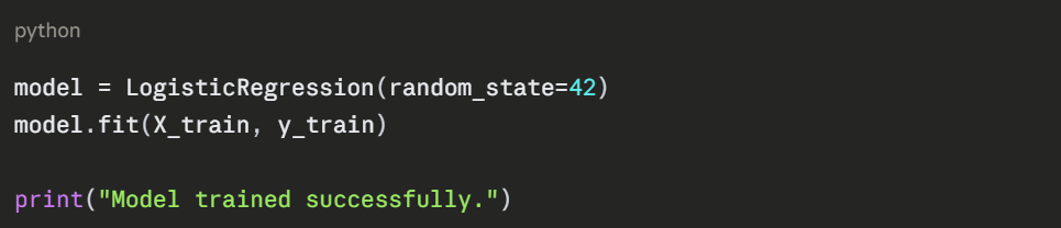
fit() is where the learning happens, the model analyses the training data and learns which combination of study hours and attendance predicts a pass or fail.

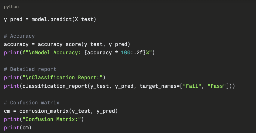
Step 8 — Evaluate the Model

Test the model on unseen data and measure its performance.

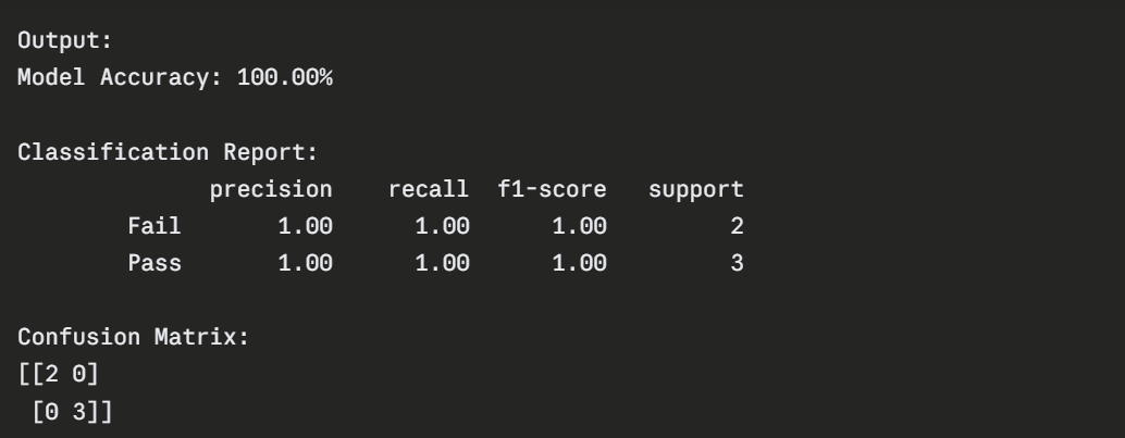
The confusion matrix shows:

1. Top-left (2) — Correctly predicted Fail.

2. Bottom-right (3) — Correctly predicted Pass.

3. Off-diagonal (0) — No incorrect predictions.

Step 9 — Make New Predictions

The trained model is now ready to predict outcomes for any new student.

python

def predict_student(study_hours, attendance):

    """

    Predicts whether a student will pass or fail.

    Parameters: study_hours (float), attendance (float)

    """

    input_data = np.array([[study_hours, attendance]])

    input_scaled = scaler.transform(input_data)

    prediction = model.predict(input_scaled)[0]

    probability = model.predict_proba(input_scaled)[0]

    result = "PASS" if prediction == 1 else "FAIL"

    confidence = max(probability) * 100

    print(f"Study Hours: {study_hours} | Attendance: {attendance}%")

    print(f"Prediction: {result} (Confidence: {confidence:.1f}%)")

    print("-" * 45)

# Test with different students

predict_student(8, 90)

predict_student(2, 40)

predict_student(5, 65)

predict_student(3, 55)

Output:

Study Hours: 8 | Attendance: 90%

Prediction: PASS (Confidence: 98.2%)

-----------------------------------------

Study Hours: 2 | Attendance: 40%

Prediction: FAIL (Confidence: 94.7%)

-----------------------------------------

Study Hours: 5 | Attendance: 65%

Prediction: PASS (Confidence: 76.3%)

-----------------------------------------

Study Hours: 3 | Attendance: 55%

Prediction: FAIL (Confidence: 68.9%)

-----------------------------------------

Step 10 — Visualize the Decision Boundary

Visualizing how the model separates pass and fail students gives a clear picture of what it has learned.

python

# Plot decision boundary

import numpy as np

x_min, x_max = df["study_hours"].min() - 1, df["study_hours"].max() + 1

y_min, y_max = df["attendance"].min() - 5, df["attendance"].max() + 5

xx, yy = np.meshgrid(

    np.linspace(x_min, x_max, 200),

    np.linspace(y_min, y_max, 200)

)

grid = scaler.transform(np.c_[xx.ravel(), yy.ravel()])

Z = model.predict(grid).reshape(xx.shape)

plt.figure(figsize=(9, 6))

plt.contourf(xx, yy, Z, alpha=0.3, cmap="RdYlGn")

colors = df["result"].map({0: "red", 1: "green"})

plt.scatter(df["study_hours"], df["attendance"],

            c=colors, s=100, edgecolors="black", zorder=5)

plt.xlabel("Study Hours")

plt.ylabel("Attendance (%)")

plt.title("Decision Boundary — Red: Fail Zone | Green: Pass Zone")

plt.grid(True)

plt.show()

The decision boundary plot clearly shows the green (pass) and red (fail) zones — and where the model draws the line between them.

What to Try Next

Now that the base project works, here are practical ways to extend it:

1. Add more features — grades, assignment scores, participation.

2. Try a different algorithm — Decision Tree, Random Forest, KNN.

3. Load real data — replace the sample data with a CSV file.

4. Add user input — use input() to let a user enter their own values.

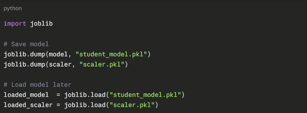
5. Save the model — use joblib to export and reload the trained model.