Pytorch
PyTorch is an open-source deep learning framework developed primarily by Facebook’s AI Research lab (FAIR). It provides a flexible and efficient platform for building and training machine learning and deep learning models. At its core, PyTorch is designed around the concept of tensors, which are multi-dimensional arrays similar to NumPy arrays but with the added capability to perform computations on GPUs for accelerated performance.
PyTorch emphasizes dynamic computation graphs, which means that the computation graph is built on-the-fly as operations are executed. This allows for greater flexibility and ease in debugging compared to static graph frameworks. Dynamic graphs make PyTorch particularly suitable for research, experimentation, and tasks where the model architecture may change during runtime, such as natural language processing or reinforcement learning.
The framework includes a rich set of modules and libraries for neural network development. The torch.nn module provides pre-built layers, loss functions, and utilities to construct complex models. torch.optim contains optimization algorithms for training models efficiently. Additionally, PyTorch integrates seamlessly with Python, allowing users to leverage standard Python tools and libraries in their workflows.
Beyond the core library, PyTorch has an ecosystem that supports model deployment, data loading, and distributed training. For example, torchvision provides datasets, models, and image transformations for computer vision tasks, while torchaudio and torchtext do the same for audio and text data. PyTorch also supports exporting models for production via TorchScript and can run on multiple platforms, including CPUs, GPUs, and mobile devices.
In essence, PyTorch is a highly flexible, efficient, and Pythonic framework for deep learning research and production, providing all the necessary tools for defining, training, and deploying advanced neural network models.
Importance of PyTorch
PyTorch is one of the leading open-source deep learning frameworks, widely used for developing AI models across research and industry. Its dynamic computational graph, intuitive API, and strong integration with Python make it particularly appealing for both experimentation and production. The importance of PyTorch lies in its flexibility, ease of use, and extensive ecosystem, which enable developers and researchers to implement complex models efficiently.
1. Dynamic Computation Graphs
PyTorch uses dynamic computation graphs, also called define-by-run graphs, which are built on the fly during execution. This allows developers to modify the network architecture, change the flow of operations, or debug models interactively without predefining the entire graph. Dynamic graphs are particularly useful in applications with variable input sizes or complex architectures, such as recurrent neural networks (RNNs) and sequence modeling. This feature distinguishes PyTorch from static-graph frameworks and makes experimentation faster and more intuitive.
2. Pythonic and Intuitive API
PyTorch is designed to be deeply integrated with Python, offering an API that feels natural for Python developers. This Pythonic approach allows the use of standard Python control flows, loops, and data structures, making model development straightforward and reducing the learning curve for beginners. Users can leverage familiar Python tools like NumPy alongside PyTorch tensors, which simplifies data manipulation and preprocessing tasks.
3. GPU Acceleration and High Performance
PyTorch provides seamless GPU support through CUDA, enabling high-speed computation of large neural networks. Operations on tensors can be executed on GPU with minimal code changes, which accelerates training and inference. This capability is essential for large-scale AI applications, including computer vision, natural language processing, and reinforcement learning, where heavy matrix computations are common.
4. Strong Ecosystem for AI Research
PyTorch has a rich ecosystem including libraries like TorchVision for computer vision, TorchText for NLP, and TorchAudio for audio processing. These libraries provide pre-built models, datasets, and utilities that simplify the development of advanced AI applications. The ecosystem also supports research experimentation, enabling rapid prototyping, model testing, and reproducibility in academic and industrial research.
5. Autograd for Automatic Differentiation
PyTorch features Autograd, an automatic differentiation system that records operations on tensors and computes gradients automatically during backpropagation. This simplifies the process of training neural networks, eliminating the need for manual gradient calculations. Autograd allows dynamic computation graphs to be differentiated in real time, which is particularly useful for complex or custom architectures where analytical gradients are difficult to derive.
6. Flexibility for Custom Model Design
PyTorch provides developers with flexibility to design custom neural network architectures, including unconventional layers, loss functions, and activation functions. This makes it ideal for research scenarios where experimentation and innovation are critical. Models can be built from scratch using the torch.nn.Module class or modified dynamically during runtime, providing complete control over the network.
7. Strong Community and Industry Adoption
PyTorch is supported by a large, active community of developers and researchers, with extensive tutorials, documentation, and forums for troubleshooting. Many academic papers and AI research projects are implemented in PyTorch, which encourages collaboration and faster adoption of new techniques. Its widespread industry adoption ensures long-term support and integration into production systems.
Uses of PyTorch
PyTorch is a versatile deep learning framework used extensively across industries for developing AI models. Its flexibility, dynamic computation, and integration with Python make it suitable for research, experimentation, and production-level applications. The following sections explain the key uses of PyTorch in various domains with detailed definitions and examples.
1. Computer Vision
PyTorch is widely used for computer vision tasks, which involve analyzing and interpreting images or videos. It supports tasks like image classification, object detection, semantic segmentation, and facial recognition. With libraries like TorchVision, developers can leverage pre-trained models, datasets, and utilities for efficient model development. PyTorch’s ability to work with GPU acceleration allows large-scale image processing tasks to be performed quickly.
Example: Self-driving cars use PyTorch to detect pedestrians, traffic signs, and vehicles in real-time to navigate safely.
2. Natural Language Processing (NLP)
PyTorch is highly effective for text-based applications, such as text classification, sentiment analysis, machine translation, and chatbots. Its support for sequence models, including RNNs, LSTMs, GRUs, and transformer architectures, makes it ideal for processing sequential data. Libraries like TorchText provide pre-processing tools, tokenization, and datasets to simplify NLP workflows.
Example: PyTorch can power a customer support chatbot that understands user queries, classifies intent, and generates appropriate responses.
3. Time Series Analysis and Forecasting
PyTorch is used to analyze time-dependent data for predicting future trends. Models such as LSTM and GRU capture temporal dependencies and patterns, making PyTorch suitable for applications like stock price prediction, energy demand forecasting, and supply chain optimization. Its dynamic graph capability allows modeling variable-length sequences efficiently.
Example: A retail company can forecast daily product demand using PyTorch, helping with inventory management and reducing overstocking.
4. Reinforcement Learning
PyTorch is extensively applied in reinforcement learning (RL), where agents learn optimal strategies by interacting with an environment and receiving feedback through rewards. RL frameworks in PyTorch facilitate the development of policy networks, value functions, and Q-learning agents. Applications include robotics, game AI, and autonomous systems.
Example: Training a robotic arm to pick and place objects efficiently using reward-based learning is implemented with PyTorch RL modules.
5. Generative Models
PyTorch is used for generative modeling, including Generative Adversarial Networks (GANs) and Variational Autoencoders (VAEs). These models create new data samples such as realistic images, videos, or text by learning underlying data distributions. PyTorch’s dynamic graph and flexible model design make it easier to experiment with complex generative architectures.
Example: GANs built with PyTorch can generate high-quality synthetic images for creative industries or data augmentation.
6. Speech Recognition and Audio Processing
PyTorch supports audio and speech-based AI applications, including speech-to-text conversion, emotion detection, and sound classification. Libraries like TorchAudio provide tools for loading, processing, and transforming audio signals. Deep learning models in PyTorch can extract features from audio waveforms and learn patterns for real-time applications.
Example: Voice assistants use PyTorch to recognize and transcribe spoken commands accurately.
7. Healthcare and Medical Imaging
PyTorch is widely applied in healthcare, particularly in analyzing medical images such as X-rays, MRIs, and CT scans. Models for disease detection, tumor segmentation, and anomaly detection are trained using PyTorch, leveraging its GPU acceleration and dynamic architecture for complex image data.
Example: PyTorch models can detect early signs of pneumonia or cancer from radiology images, assisting doctors in diagnosis.
PyTorch Tensors and Operations
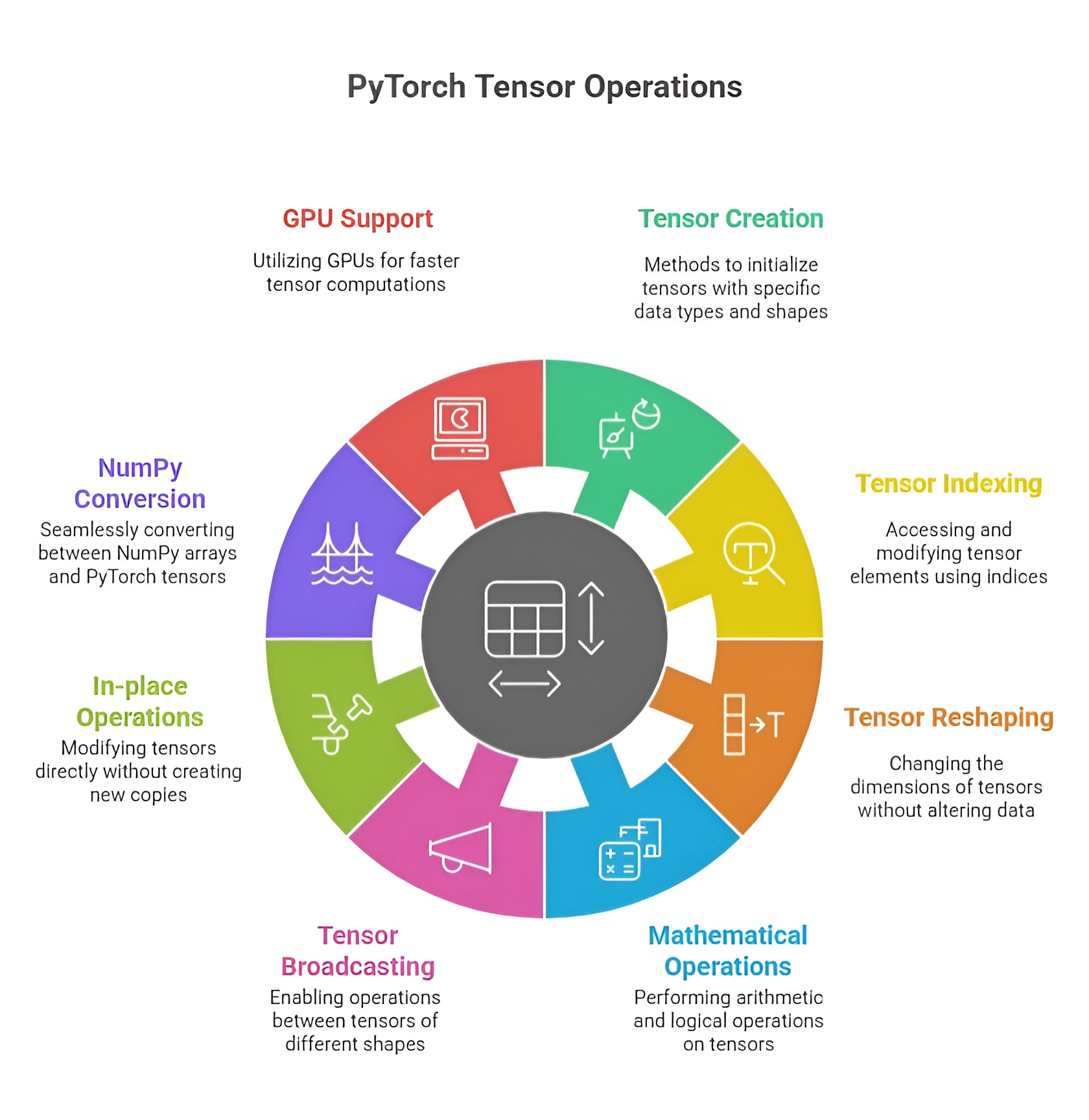
Tensors are the core data structures in PyTorch, analogous to multi-dimensional arrays in NumPy but with additional capabilities like GPU acceleration and automatic differentiation. They are the building blocks for neural networks and AI computations, representing scalars, vectors, matrices, or higher-dimensional datasets. Understanding tensor creation, attributes, operations, indexing, reshaping, and conversion is crucial for efficient deep learning workflows.
1. Creating Tensors
PyTorch provides multiple ways to create tensors based on the required initialization or data type. Tensors can be initialized with zeros, ones, or random values. torch.zeros creates a tensor filled with zeros, often used as placeholders or initial states in models, while torch.ones fills the tensor with ones, commonly used to initialize bias parameters. Random tensors are created with torch.rand, generating uniform values between 0 and 1, or torch.randn, producing values from a standard normal distribution, which are often used for weight initialization to break symmetry. For sequential or evenly spaced data, torch.arange produces values in a specified range with a fixed step, and torch.linspace generates a set number of evenly spaced points over a range, useful for time steps, grids, or input features.
Example:
import torch
zeros_tensor = torch.zeros(2, 3) # 2x3 tensor of zeros
ones_tensor = torch.ones(3, 2) # 3x2 tensor of ones
random_tensor = torch.rand(2, 2) # random uniform values
sequence_tensor = torch.arange(0, 10) # 0 to 9
linspace_tensor = torch.linspace(0, 1, 5) # 5 points between 0 and 1
2. Tensor Attributes
Every tensor has important attributes that describe its structure and properties. The shape attribute gives the dimensions of the tensor, which is essential for ensuring compatibility between layers in neural networks. The dtype attribute indicates the data type of elements, such as float32 or int64, affecting precision and memory usage. The device attribute specifies whether the tensor is on the CPU or GPU, allowing efficient computation on hardware accelerators. Inspecting these attributes helps developers debug, optimize, and design compatible model architectures.
Example:
print(zeros_tensor.shape) # Output: torch.Size([2, 3])
print(random_tensor.dtype) # Output: torch.float32
print(ones_tensor.device) # Output: cpu (or cuda:0 if on GPU)
3. Tensor Operations
PyTorch tensors support a wide variety of operations. Basic arithmetic includes addition, subtraction, multiplication, and division, which can be performed element-wise between tensors of compatible shapes. More advanced operations such as matrix multiplication, exponentiation, and trigonometric functions are also supported. These operations are optimized for CPU and GPU execution, enabling large-scale computations. Operations can be performed in-place or produce new tensors depending on requirements.
Example:
a = torch.tensor([1, 2, 3])
b = torch.tensor([4, 5, 6])
sum_tensor = a + b # element-wise addition
product_tensor = a * b # element-wise multiplication
matmul_tensor = torch.matmul(a.view(1, 3), b.view(3, 1)) # matrix multiplication
4. Indexing, Slicing, and Reshaping
Indexing allows access to individual elements, rows, or columns of a tensor. Slicing enables extraction of sub-tensors along one or more dimensions. Reshaping changes the dimensions of a tensor without modifying its underlying data, which is essential for matching input shapes to neural network layers. Methods like view, reshape, and permute allow flexible rearrangement of tensor data for computation or visualization.
Example:
tensor = torch.arange(9).view(3, 3)
element = tensor[1, 2] # access element at row 1, column 2
row_slice = tensor[0, :] # first row
reshaped = tensor.view(1, 9) # reshape to 1x9 tensor
5. Converting Between NumPy Arrays and PyTorch Tensors
PyTorch tensors can be easily converted to and from NumPy arrays, allowing integration with Python’s scientific ecosystem. Using torch.from_numpy, a NumPy array is converted into a tensor while sharing memory, so changes in one are reflected in the other. Conversely, .numpy() converts a tensor to a NumPy array for further processing, visualization, or compatibility with other libraries like Pandas or Matplotlib.
Example:
import numpy as np
np_array = np.array([1, 2, 3])
tensor_from_np = torch.from_numpy(np_array)
tensor_to_np = tensor_from_np.numpy()
PyTorch tensors provide efficient, flexible, and GPU-compatible data structures for deep learning. Their creation methods, rich attributes, versatile operations, indexing and reshaping capabilities, and seamless NumPy integration make them essential for building, training, and deploying neural network models. Understanding these fundamentals allows developers to manipulate data effectively, design complex architectures, and leverage the full potential of PyTorch for AI applications.
Autograd and Gradients in PyTorch
PyTorch provides Autograd, a dynamic automatic differentiation system that records operations performed on tensors with requires_grad=True to create a computation graph. This graph stores the relationship between inputs and outputs, enabling automatic computation of derivatives, which is essential for gradient-based optimization in neural networks. Tensors that require gradients are usually model parameters like weights and biases, while tensors without gradient tracking are treated as constants.
1. Creating Tensors and Setting requires_grad
Tensors in PyTorch can be created with requires_grad=True to indicate that operations on them should be tracked for gradient computation. For instance, x = torch.tensor(2.0, requires_grad=True) will record all operations for later differentiation, whereas a tensor y = torch.tensor(3.0) will not participate in gradient tracking. This selective tracking optimizes memory usage and computation efficiency.
import torch
x = torch.tensor(2.0, requires_grad=True)
y = torch.tensor(3.0)
print(x.requires_grad) # True
print(y.requires_grad) # False
2. Performing Operations and Building the Computation Graph
Operations on tensors with requires_grad=True automatically construct a computation graph. This graph dynamically maps how outputs depend on inputs, enabling backward propagation of gradients. For example, performing z = x**2 + 3*x creates a graph that records the sequence of operations needed to compute the derivative with respect to x.
z = x**2 + 3*x
print(z) # 10.0
3. Computing Gradients with .backward()
Gradients of scalar tensors can be computed automatically using the .backward() method. PyTorch calculates derivatives for all tensors in the computation graph with requires_grad=True and stores them in the .grad attribute. For example, calling z.backward() computes the derivative dz/dx = 2*x + 3 and stores it in x.grad.
z.backward()
print(x.grad) # 7.0
4. Gradient Accumulation and Zeroing
PyTorch accumulates gradients by default across multiple backward passes. To prevent incorrect updates during iterative training, gradients must be reset using x.grad.zero_() before each new computation. For example, after computing z = x**3 and calling .backward(), the gradient accumulates to 19.0 (previous 7 + 12 from derivative 3*x**2). Resetting gradients ensures accurate parameter updates.
z = x**3
z.backward()
print(x.grad) # 19.0
x.grad.zero_()
print(x.grad) # 0.0
5. Using torch.no_grad() During Inference
During evaluation or inference, gradient computation is unnecessary. Wrapping computations inside with torch.no_grad(): disables gradient tracking, reducing memory usage and improving execution speed. This allows for efficient predictions without affecting previously computed gradients.
with torch.no_grad():
z_eval = x**2 + 3*x
print(z_eval) # 10.0
print(x.grad) # 0.0
6. Full Practical Workflow Example
A complete workflow demonstrates the typical usage of Autograd in training and inference. First, tensors are created with requires_grad=True. Forward computations are performed, and gradients are automatically calculated using .backward(). Gradients are reset between iterations to prevent accumulation errors. Inference is executed efficiently without tracking gradients using torch.no_grad().
x = torch.tensor(2.0, requires_grad=True)
y = x**2 + 3*x
y.backward()
print(f"Gradient after first backward: {x.grad}") # 7.0
x.grad.zero_()
y_new = x**3 + 2*x
y_new.backward()
print(f"Gradient after second backward: {x.grad}") # 14.0
with torch.no_grad():
y_infer = x**2 + 5*x
print(f"Inference output: {y_infer}") # 14.0
Autograd in PyTorch provides a dynamic, flexible, and efficient framework for automatic differentiation, allowing developers to implement neural network training workflows with precision. By combining tensors with requires_grad, automatic gradient computation, gradient accumulation management, and inference without gradient tracking, PyTorch simplifies complex optimization tasks. This system is fundamental for research, experimentation, and real-world deep learning applications, eliminating the need for manual derivative calculations and improving both memory efficiency and computational speed.
Neural Networks in PyTorch
1. What is a Neural Network?
A neural network is a computational model inspired by the human brain, consisting of interconnected nodes called neurons arranged in layers. Each neuron receives inputs, applies a weighted sum, passes it through an activation function, and produces an output. Neural networks can learn complex relationships from data, making them essential for deep learning tasks such as image classification, natural language processing, and reinforcement learning. They can model non-linear functions, detect patterns, and generalize knowledge from training data to unseen inputs.
2. Introduction to torch.nn Module
The torch.nn module in PyTorch provides tools for defining and building neural networks. It allows developers to create layers, combine them into networks, and automatically track parameters for training. Layers like nn.Linear represent fully connected layers, while modules like nn.Sequential can stack multiple layers in order. The nn.Module base class is used to define custom networks by specifying the forward computation. The module also integrates seamlessly with loss functions and optimizers, allowing easy forward and backward passes for training.
3. Building Simple Feedforward Neural Networks
A simple feedforward neural network consists of an input layer, one or more hidden layers, and an output layer. Each hidden layer applies a non-linear activation function, enabling the network to learn complex patterns. Using nn.Linear, developers define layers that automatically handle weights and biases. The forward pass involves passing input data through the layers sequentially, applying activation functions at hidden layers, and computing output at the final layer. Backpropagation is then used to compute gradients and update weights using optimizers.
import torch
import torch.nn as nn
import torch.optim as optim
class SimpleNN(nn.Module):
def __init__(self, input_size, hidden_size, output_size):
super(SimpleNN, self).__init__()
self.fc1 = nn.Linear(input_size, hidden_size)
self.relu = nn.ReLU()
self.fc2 = nn.Linear(hidden_size, output_size)
def forward(self, x):
out = self.fc1(x)
out = self.relu(out)
out = self.fc2(out)
return out
model = SimpleNN(input_size=3, hidden_size=5, output_size=1)
4. Activation Functions (ReLU, Sigmoid, Tanh)
Activation functions introduce non-linearity into neural networks, allowing them to approximate complex functions. ReLU (Rectified Linear Unit) outputs zero for negative inputs and the input itself for positive values, preventing vanishing gradient problems and speeding up training. Sigmoid maps input values between 0 and 1, which is suitable for binary classification outputs. Tanh maps input values between -1 and 1, providing a zero-centered activation. Choosing the right activation function affects learning efficiency and network performance.
relu = nn.ReLU()
sigmoid = nn.Sigmoid()
tanh = nn.Tanh()
x = torch.tensor([-1.0, 0.0, 2.0])
print(relu(x)) # Output: tensor([0., 0., 2.])
print(sigmoid(x)) # Output: tensor([0.2689, 0.5, 0.8808])
print(tanh(x)) # Output: tensor([-0.7616, 0.0000, 0.9640])
5. Forward Pass, Backward Pass, and Loss Computation
The forward pass computes the output of the network by passing inputs through each layer and applying activation functions. The loss function quantifies the difference between predicted outputs and target values, guiding the learning process. Common loss functions in PyTorch include nn.MSELoss for regression and nn.CrossEntropyLoss for classification. During the backward pass, PyTorch automatically computes gradients for all trainable parameters using Autograd. Optimizers, such as SGD or Adam, then update the weights and biases based on these gradients. This cycle of forward pass, loss computation, backward pass, and weight update is repeated over multiple epochs to train the network.
criterion = nn.MSELoss()
optimizer = optim.SGD(model.parameters(), lr=0.01)
inputs = torch.tensor([[1.0, 2.0, 3.0]])
target = torch.tensor([[1.0]])
outputs = model(inputs) # Forward pass
loss = criterion(outputs, target)
optimizer.zero_grad() # Reset gradients
loss.backward() # Backward pass
optimizer.step() # Update weights
6. Integrated Workflow
In practice, the training workflow involves defining a network with nn.Module, choosing activation functions for hidden layers, computing outputs in the forward pass, measuring errors using a loss function, calculating gradients automatically through .backward(), and updating parameters with an optimizer. This process allows neural networks to learn from data efficiently while abstracting away manual gradient calculations. By repeating this process for multiple iterations, the network gradually improves its predictions and generalizes patterns from training data to unseen inputs.
Training a Model in PyTorch
Training a model in PyTorch involves creating a neural network, preparing data, performing forward and backward passes, updating parameters using an optimizer, and monitoring performance metrics such as loss and accuracy. The training process is iterative, allowing the model to learn patterns from data over multiple epochs. PyTorch provides flexible tools for data handling, model definition, gradient computation, and checkpointing, which streamline the workflow for both research and practical applications.
1. Steps to Train a PyTorch Model
The typical workflow for training a PyTorch model starts with defining the neural network architecture, choosing a suitable loss function, and selecting an optimizer. Next, data is prepared and batched, and the training loop is executed over multiple epochs. Within each iteration, the model performs a forward pass to compute predictions, calculates the loss, computes gradients using Autograd, and updates parameters via the optimizer. After training, models can be evaluated, saved, and reloaded for future use. This structured approach ensures reproducible and efficient training of neural networks.
import torch
import torch.nn as nn
import torch.optim as optim
# Define a simple neural network
class SimpleNN(nn.Module):
def __init__(self):
super(SimpleNN, self).__init__()
self.fc1 = nn.Linear(2, 4)
self.fc2 = nn.Linear(4, 1)
def forward(self, x):
x = torch.relu(self.fc1(x))
x = self.fc2(x)
return x
model = SimpleNN()
criterion = nn.MSELoss()
optimizer = optim.SGD(model.parameters(), lr=0.01)
2. Data Preparation and Batching
Data preparation is crucial for training stability and efficiency. Inputs and targets are converted to PyTorch tensors, normalized if needed, and organized into batches using DataLoader. Batching allows the model to process multiple samples simultaneously, reducing computation time and improving gradient estimation. Shuffling the data ensures that the model does not learn patterns based on the order of samples.
from torch.utils.data import DataLoader, TensorDataset
# Sample data
X = torch.tensor([[1.0, 2.0], [3.0, 4.0], [5.0, 6.0], [7.0, 8.0]])
y = torch.tensor([[3.0], [7.0], [11.0], [15.0]])
dataset = TensorDataset(X, y)
dataloader = DataLoader(dataset, batch_size=2, shuffle=True)
3. Implementing Epochs and Training Loops
Training is performed over multiple epochs, where each epoch represents one complete pass through the entire dataset. Within each epoch, batches are processed sequentially. For every batch, the model performs a forward pass to generate predictions, computes the loss, executes a backward pass to calculate gradients, and updates the model parameters using the optimizer. This iterative process gradually reduces the loss, allowing the model to learn from the data.
epochs = 5
for epoch in range(epochs):
for batch_X, batch_y in dataloader:
optimizer.zero_grad() # Reset gradients
outputs = model(batch_X) # Forward pass
loss = criterion(outputs, batch_y) # Compute loss
loss.backward() # Backward pass
optimizer.step() # Update parameters
print(f"Epoch [{epoch+1}/{epochs}], Loss: {loss.item():.4f}")
4. Tracking Training Loss and Accuracy
Monitoring training metrics such as loss and accuracy is essential to evaluate model performance and detect issues like underfitting or overfitting. Loss provides a measure of prediction error, while accuracy (for classification tasks) reflects how often the model predicts the correct class. These metrics can be logged after each batch or epoch to visualize learning progress over time.
# Example: tracking simple training loss
for epoch in range(epochs):
total_loss = 0
for batch_X, batch_y in dataloader:
optimizer.zero_grad()
outputs = model(batch_X)
loss = criterion(outputs, batch_y)
loss.backward()
optimizer.step()
total_loss += loss.item()
avg_loss = total_loss / len(dataloader)
print(f"Epoch [{epoch+1}/{epochs}], Average Loss: {avg_loss:.4f}")
5. Saving and Loading Models
PyTorch allows models to be saved and loaded efficiently using torch.save and torch.load. Saving the state dictionary of the model preserves trained weights, enabling later reuse or deployment without retraining. Models can be reloaded into the same architecture or transferred to new environments for inference or further training.
# Save model state
torch.save(model.state_dict(), "simple_model.pth")
# Load model state
loaded_model = SimpleNN()
loaded_model.load_state_dict(torch.load("simple_model.pth"))
loaded_model.eval() # Set to evaluation mode
Training a PyTorch model integrates data preparation, batching, iterative training loops, gradient computation, and parameter updates into a systematic workflow. By tracking metrics like loss and accuracy, developers can ensure effective learning, while saving and loading models provides flexibility for deployment and experimentation. This end-to-end process underpins deep learning applications, enabling reproducible, scalable, and efficient model training and inference.
Convolutional Neural Networks (CNNs) in PyTorch
1. Introduction to CNNs and Their Importance
Convolutional Neural Networks, or CNNs, are a specialized class of neural networks designed to process data with a grid-like topology, such as images. Unlike traditional fully connected networks, CNNs leverage spatial hierarchies by applying convolutional filters to detect features like edges, textures, and shapes. This makes CNNs highly effective for image-related tasks, including classification, object detection, and segmentation. CNNs reduce the number of parameters compared to fully connected networks, improving computational efficiency and allowing the model to capture local patterns in images that are critical for accurate predictions.
2. Convolutional Layers and Pooling Layers
A convolutional layer applies a set of learnable filters (kernels) across the input image to extract features. Each filter slides over the input, performing element-wise multiplications and summing the results to create feature maps that highlight specific patterns. Convolutional layers can be stacked to capture increasingly complex features at deeper layers. A pooling layer reduces the spatial dimensions of feature maps, summarizing regions of the input to make the network less sensitive to spatial variations and to reduce computational load. Common pooling operations include max pooling, which selects the maximum value in a region, and average pooling, which computes the average. Combining convolutional and pooling layers allows CNNs to progressively extract and condense information from images.
3. Building a Simple CNN in PyTorch
In PyTorch, CNNs are implemented using the torch.nn module. Convolutional layers are created with nn.Conv2d, pooling layers with nn.MaxPool2d or nn.AvgPool2d, and fully connected layers with nn.Linear. Activation functions like ReLU are applied after convolutional layers to introduce non-linearity. A typical CNN consists of a sequence of convolutional and pooling layers followed by fully connected layers for classification. The forward pass defines how input images flow through these layers to produce outputs.
import torch
import torch.nn as nn
import torch.optim as optim
# Define a simple CNN
class SimpleCNN(nn.Module):
def __init__(self, num_classes=10):
super(SimpleCNN, self).__init__()
self.conv1 = nn.Conv2d(in_channels=1, out_channels=16, kernel_size=3, stride=1, padding=1)
self.relu = nn.ReLU()
self.pool = nn.MaxPool2d(kernel_size=2, stride=2)
self.conv2 = nn.Conv2d(16, 32, 3, 1, 1)
self.fc1 = nn.Linear(32 * 7 * 7, 128)
self.fc2 = nn.Linear(128, num_classes)
def forward(self, x):
x = self.conv1(x)
x = self.relu(x)
x = self.pool(x)
x = self.conv2(x)
x = self.relu(x)
x = self.pool(x)
x = x.view(x.size(0), -1) # Flatten feature maps
x = self.fc1(x)
x = self.relu(x)
x = self.fc2(x)
return x
model = SimpleCNN(num_classes=10)
4. Using CNN for Image Classification Tasks
CNNs are widely used for image classification, where the goal is to assign a label to each input image. Images are passed through the convolutional and pooling layers to extract features, which are then flattened and fed into fully connected layers to produce class probabilities. PyTorch’s nn.CrossEntropyLoss is commonly used for multi-class classification, while optimizers like SGD or Adam update network weights during training. A forward pass computes predictions, the loss function measures errors, and backpropagation calculates gradients for optimization. After multiple epochs of training, the CNN learns to recognize patterns and classify new, unseen images accurately.
# Example forward pass and loss computation
criterion = nn.CrossEntropyLoss()
optimizer = optim.Adam(model.parameters(), lr=0.001)
# Sample input: batch of grayscale images of size 28x28
inputs = torch.randn(8, 1, 28, 28)
targets = torch.randint(0, 10, (8,))
# Forward pass
outputs = model(inputs)
loss = criterion(outputs, targets)
# Backward pass and optimization
optimizer.zero_grad()
loss.backward()
optimizer.step()
In this example, inputs represent a batch of 8 grayscale images of size 28x28, and targets are the corresponding class labels. The CNN extracts features through convolutional and pooling layers, produces predictions, computes the classification loss, and updates weights through backpropagation.
CNNs in PyTorch provide a structured and efficient framework for image-related tasks, combining convolutional layers, pooling layers, and fully connected layers to capture spatial features and make accurate predictions. By leveraging Autograd for automatic differentiation and the torch.nn module for layer management, developers can build and train CNNs effectively for real-world applications such as digit recognition, object detection, and facial recognition.